Computational Ants: Agent Based Visualization Technique with CDR OD Matrix

by Ira Winder and Nina Lutz

Introduction

So you want to make a granular model of a system, but you don't think you have all of the data you need? This is actually a very common situation in modeling. Before going on a quest to search for more data, I often remind researchers that a good model might not need as much data as they think.

To demonstrate, let's review a technique called "agent based visualization," a data-light technique for modeling flows of people using a simple and common data set called an origin-destination matrix (OD matrix, for short).

What is an Origin-Destination Matrix?

Trip behavior data is often collected as an OD matrix. An OD matrix reflects aggregate flows between a number of discrete locations over a period of time (Fig. 1).

Figure 1. A conceptual diagram of an origin-destination matrix. Source: Dr. Jean-Paul Rodrigue, Dept. of Global Studies & Geography , Hofstra University, New York, USA.

For our exercise, we'll use a 2D environment created in Processing. An OD matrix is randomly generated (Fig. 2 and 3). In a simple visualization, trip counts are represented by lines connecting points. Larger counts are represented by thicker lines. Color in Fig. 3 is arbitrary but unique to each OD pair.

Figure 2. Randomly generated origin-destination pairs. Image: Ira Winder

Figure 3. Randomly generated OD matrix. Image: Ira Winder

That's great, but now we want to tease out some additional information. In particular, we want a better understanding of directionality and routing within our OD matrix. First, we'll tackle directionality using agent-based modeling techniques. Solid lines are replaced with continuous flows of individual agents (Fig 4).  

By animating the network, we have a bit better understanding of flow, particularly directionality. The total amount of agents flowing between two points at any given time is proportional to the flow defined in the OD matrix. Keep in mind, however, that time is an abstract dimension in this visualization. Motion and speed are in fact arbitrary constructs that only serve to make our OD matrix more human-readable. The quantity of agents on the screen, however, is not arbitrary. Rather, quantity of agents is the key parameter by which we communicate information from our OD matrix.

Figure 4. Agent-based modeling technique that communicates relative flow and directionality of a random OD matrix. Image: Ira Winder

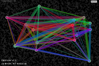
Figure 5. Pathfinding algorithm applied to approximate routing. Image: Ira Winder

Now that we've tackled directionality, we'll try to tackle the issue of routing. You've probably noticed that OD matrices tell us nothing of how one travels from point A to point B. While visualizing the routes as straight-shot lines is easy, it is hardly realistic (except for the birds, perhaps). A pathfinding algorithm, such as Dijkstra's, can be helpful for solving this. We've randomly generated a "road" network for our model, lightly colored in gray. The agents are now programmed to take the shortest route along the network provided (Fig. 5). Not only does our visualization show a more realistic representation of routing, it starts to reveal emergent "corridors" where traffic, and perhaps congestion, might be prevalent. However, any observations at this point are purely qualitative.

If you'd like to view an implementation of pathfinding in Processing, go to my repository.

Poly-Voxels

By the way, you might have noticed that our example uses a poly-voxel network (Fig. 6a and 6b). This is mostly an arbitrary preference. It might make sense, however, given some of our other projects.

Figure 6a. Voxel-based data abstraction. Image: Ira Winder

Figure 6b. A poly-voxel network with shortest-paths between origins and destinations highlighted. Image: Ira Winder

Network Design

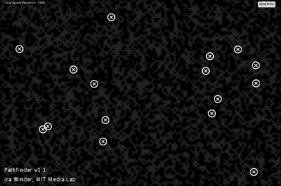
Despite all my talk of minimizing the need for data, you might point out that even a routing algorithm requires data for a road network. Touché. In the example above, we've randomly generated data for a network, but you might want to model a specific network yourself. We've created a couple tools to help with that. One tool let's you manually "sketch" a valid network by drawing obstacles (Fig. 7). We imagine this technique might be useful if you lack vector data but can get ahold of a raster/satellite image.

Figure 7. A custom network is created by subtracting polygons from the field. Image: Ira Winder

Figure 8a. Agent-based visualization of pedestrian activity between amenities. Image: Ira Winder

In most cases, though, road vector data is available from various sources such as Open Street Maps. We made a utility that converts such road vector data into our poly-voxel format (Fig. 8b). There's no particular reason you couldn't use vectors directly from OSM, but we prefer the sketchy-ness of the poly-voxels to emphasize the roughness of our approximations. We tested the OSM network by modeling pedestrian movement between amenities (Fig. 8a).

Figure 8b.  GIS Vector data (left) translated into poly-voxel data (right).  The translation differentiates between different path types such as roads, sidewalks, and pedestrian bridges. The purple network is an elevated walkway.

Implementation

Our primary implementation for this model was for visualization of call detail records (CDR) for the City of Andorra la Vella (Fig. 9a). CDRs can be converted into a type of OD matrix where origins and destinations are represented by cell phone towers. The transition from one tower to the next is captured when a user's cell phone signal switches from one tower to another. This transition is called a handoff and can be the source of a very rich OD matrix.

You can see the code for this implementation in this Github repository.

Figure 9a: Andorra CDR OD Matrix from Cirque du Solei dataset, representing 1 hour of calls handed off between cell towers. Viedo: Nina Lutz

One issue with our visualization thus far is the use of cell phone towers as our literal origins and destinations. In reality, people do not travel to and from cell phone towers but rather to the amenities and homes within their coverage. Using a Voronoi technique, we can determine roughly which Andorran amenities are associated with each cell tower (Figure 9b). This is, of course, a very rough approximation.

Figure 9b. Voronoi method used to allocate cell phone tower data to surrounding amenities. Image: Nina Lutz

Figure 9c. Agent-based visualization of Spanish-speaking (orange) and French-speaking (blue) tourists of Andorra la Vella using CDR data, Amenities, and road network data. Image: Nina Lutz

The result is a more nuanced visualization with trips that begin and end at valid amenity locations (Fig. 9c).The methodology was also adapted for a tangible interactive model of pedestrian activity of a Singaporean neighborhood (Figure 10). Users can adjust an OD matrix by configuring pieces that represent amenities.

Figure 10. A bus stop, represented by two red circles, is not within walking distance of nearby amenities (left). Amenities placed within walking distance of the bus stop increase simulated pedestrian activity in the areas (right). Image: Ira Winder

The term "Agent Based Visualization" appears in other literature including, but not limited to:

• Hagen, Hans et al. "A Component and Multi Agent-based Visualization System Architecture." ICM, 2000
• Roard, Nicolas and Jones, Mark M. "Agent Based Visualization and Strategies." 30 January, 2006.
• Grignard, Arnaud et al. "Agent-Based Visualization: A Simulation Tool for the Analysis of River Morphosedimentary Adjustments." Multi-Agent Based Simulation XVI15 March 2016.